Machine Learning for MRI Image Reconstruction
Discuss this piece on Hacker News or Twitter.
Magnetic resonance imaging (MRI) has long scan times, sometimes close to an hour for an exam. This sucks because long scan times makes MRI exams more expensive, less accessible, and unpleasant. [How does it feel like to be in an MRI?]
Here, I review some methods in machine learning that aim to reduce the scan time through new ways of image reconstruction. Smarter image reconstruction allows us to acquire way less data, which means shorter scan times. These techniques are pretty general and can be applied to other image reconstruction problems.
Disclaimer: This is not meant to be a comprehensive review. Rather, it is just a sample of some methods I found cool.
MRI Image Reconstruction
In most medical imaging methods, what you see on the screen isn’t just a raw feed of what the device’s sensors are picking up.
In MRI, this is what the sensors pick up:
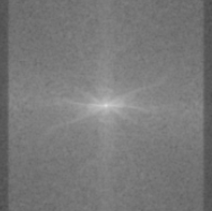
How in the world is this data useful? Image reconstruction is this incredible procedure that can turn this mess of sensor data into an actual image. After doing image reconstruction on the sensor data above, we get:
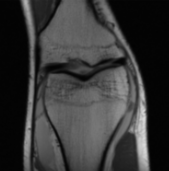
Now that’s much better! (this is an MRI of the knee.) So how does this magical procedure of turning sensor data into images work?
A nice way to frame this problem is to consider the signals the sensors pick up as a mathematical transformation of the image. In this framing, creating an image is inverting this mathematical transformation. This might seem backward, but it’ll become handy soon.
In MRI, the transformation from image to sensor data is a 2D or 3D Fourier transform. This is super wacky! It means the sensors somehow measure the spatial frequencies in the image1! We can write this as:
$$ \mathbf{y} = \mathcal{F} (\mathbf{x}^*) $$
where $ \mathbf{y} $ is the (noiseless) sensor data, $\mathbf{x}^* $ is the ground-truth image, and $\mathcal{F}$ is the Fourier transform.
Reconstructing the image from the frequency-domain (sensor) data is simple: we just apply an inverse Fourier transform. $$ \mathbf{\hat{x}} = \mathcal{F}^{-1}(\mathbf{y}) $$
(Note, we’re assuming that we’re recording from a single MRI coil with uniform sensitivity, but these methods can be extended to multi-coil imaging with non-uniform sensitivity maps.)
Using Less Data
The MRI Gods (linear algebra) tell us that if we want to reconstruct an image with $n$ pixels (or voxels), we need at least $n$ frequencies. [Why?]
But the problem with acquiring $n$ frequencies is that it takes a lot of time. This is because MRI scan time scales linearly with the number of frequencies you acquire2. A typical MRI image has on the order of 10 million frequencies, which – even with many hardware and software tricks to cut acquisition time – means an MRI exam typically takes ~40 minutes and can sometimes take as long as an hour. If we could acquire only 1/4th of the frequencies, we can reduce acquisition time by 4x (and therefore MRIs could cost 4x less).
So suppose we drink a bit too much and forget about the linear algebra result, only acquiring a subset of the frequencies. Let’s set the data at the frequencies that we didn’t acquire to be 0. We can write this as
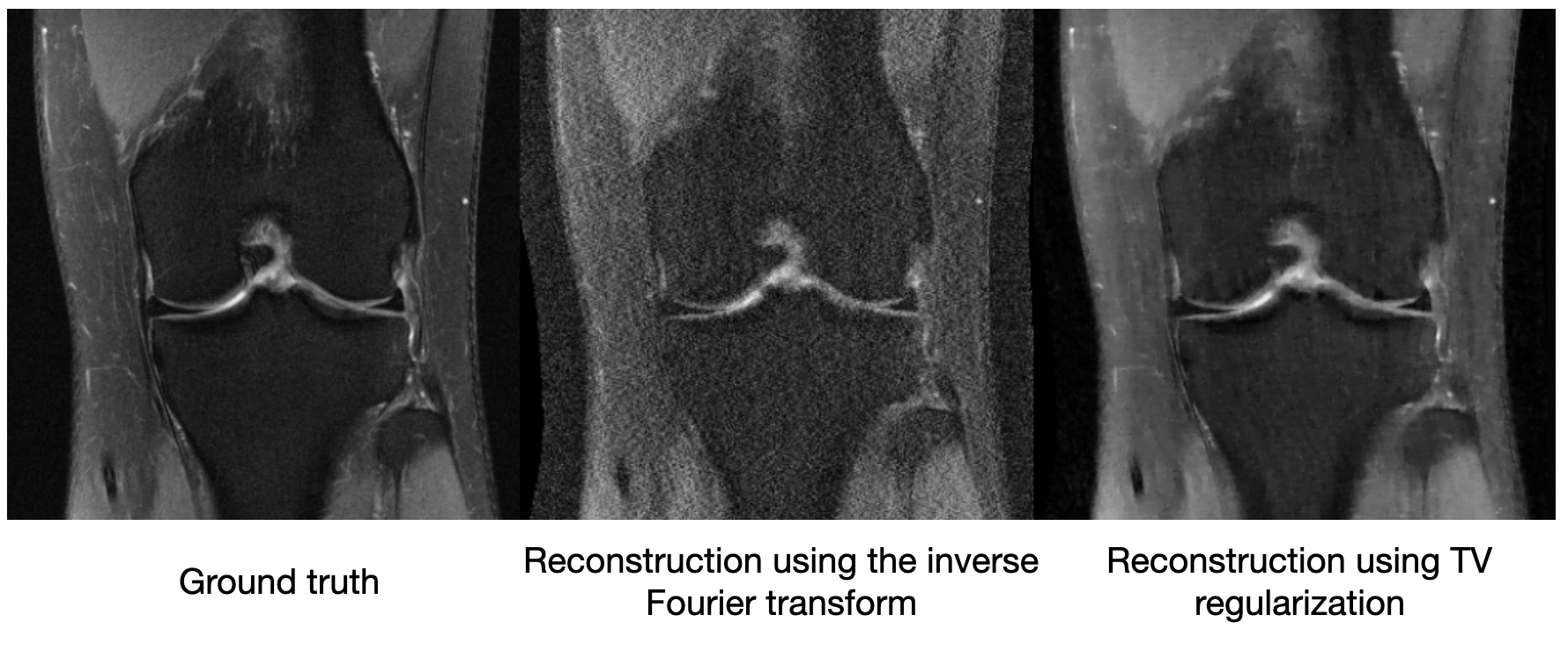
$$\mathbf{\tilde{y}} = \mathcal{M} \odot \mathbf{y} = \mathcal{M} \odot \mathcal{F} (\mathbf{x}^*)$$ where $\mathcal{M}$ is a masking matrix filled with 0s and 1s, and $\odot$ denotes element-wise multiplication. If we try to reconstruct the same knee MRI data as above with less frequencies, we get (aliasing) artifacts:
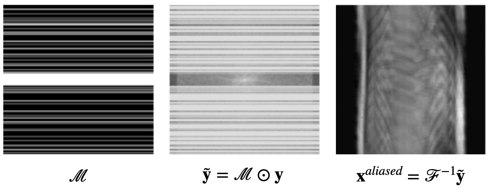
So our dreams of using less frequencies are over, right?
What if we add more information to the image reconstruction process that is not from the current measurement $\mathbf{\tilde{y}} $? For example, in compressed sensing, we can assume that the desired image $\mathbf{x}$ doesn’t have many edges (i.e., that we can “compress” the edges). Here’s a knee MRI along with its edge map, which we see is very sparse:
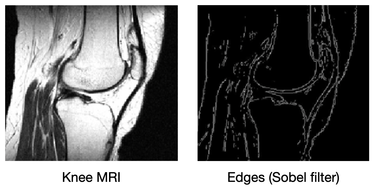
How do we incorporate the fact that we know that MRI images aren’t supposed to have many edges? First, we need some way of counting how many edges are in an MRI image. Edges are places in the image with high spatial derivatives, so a decent way to count edges is by summing the spatial derivatives (this is called the total variation, and we can write this mathematically as $R_{TV}(\mathbf{x}) = ||\nabla \mathbf{x}||_1$, where $\nabla$ is the spatial gradient and $||.||_1$ is the L1 norm).
It isn’t enough to just look for images that are not so edgy though; we still need our images to match the measurements that we collect (otherwise, we can just make our image blank). We can combine these two components into the following optimization problem: $$ \argmin_{\mathbf{x}} || \mathcal{M} \odot \mathcal{F}(\mathbf{x}) - \mathbf{\tilde{y}} ||_2^2 + R _{TV}(\mathbf{x}) $$
where $ || . ||_2 $ is the L2 norm (i.e., $||z||_2^2 = \sum_i |z_i|^2 $). The left term says: “If $\mathbf{x}$ were the real image, how would the sensor data we’d capture from $\mathbf{x}$ compare with our real sensor data $\mathbf{\tilde{y}}$?” In other words, it tells us how much our reconstruction $\mathbf{x}$ agrees with our measurements $\mathbf{\tilde{y}}$. The right term $R _ {TV} (\mathbf{x})$ penalizes images if they are too edgy. The challenge is finding an image that both agrees with our measurements and isn’t too edgy. Algorithms like gradient descent allows us to solve the optimization problem above. [What is gradient descent?]
Though compressed sensing can improve the image quality relative to a vanilla inverse Fourier transform, it still suffers from artifacts. We see below on a 4x subsampled knee MRI that TV regularization makes some improvements over the inverse Fourier transform (source):
Maybe just saying “MRI images shouldn’t be very edgy” isn’t enough information to cut the sensor data by a factor of 4. So other methods of compressed sensing might say “MRI images should be sparse” or “MRI images should be sparse in a wavelet basis.” These methods do this by replacing $R_{TV}(\mathbf{x})$ with a more general $R(\mathbf{x})$, which we call a regularizer. The difficulty with classical compressed sensing is that humans must manually encode what an MRI should look like through the regularizer $R(\mathbf{x})$. We can come up with basic heuristics like the examples above, but ultimately deciding whether an image looks like it could have come from an MRI is a complicated process. [How do you interpret R(x) using information theory?]
Enter machine learning… Over the past decade-ish, machine learning has had great success in learning functions that humans have difficulty hard coding. It has revolutionized the fields of computer vision, natural language processing, among others. Instead of hard coding functions, machine learning algorithms learn functions from data. In the next section, we will explore a few recent machine learning approaches to MRI image reconstruction.
[Did you know Terence Tao was one of the pioneers of compressed sensing?]Machine Learning Comes to the Rescue
A Naive Approach
We can throw a simple convolutional neural network (CNN) at the problem. [What is a convolutional neural network?]
The CNN could take in the sensor measurements $\mathbf{\tilde{y}}$ and output its predicted image $\mathbf{\hat{x}}$3. After collecting a dataset that includes both measurements $\mathbf{\tilde{y}}$ and properly reconstructed images $\mathbf{{x}^*}$, you can train the neural network to make its predicted images as close to the ground truth images.
The problem with this approach is that we don’t tell the neural network anything about the physics of MRI. This means it has to learn to do MRI image reconstruction from scratch, which will require a lot of training data.
U-Net MRI
How can we tell our machine learning method about the physics of MRI image reconstruction? One idea is to first turn the sensor data into an image via an inverse Fourier transform before feeding it into a CNN. Now, the CNN would just have to “clean up” what was missed by the inverse Fourier transform. This is the approach taken by U-Net MRI, where the CNN is chosen to be a U-Net. U-Nets are a popular image-to-image model for biomedical applications.
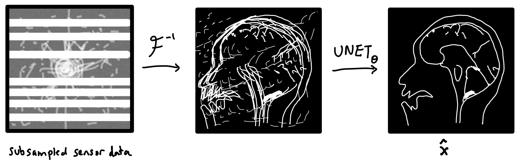
We can formally write the operations performed by this network as $$ \mathbf{\hat{x}} = \text{UNET}_{{\boldsymbol{\theta}}}(\mathcal{F}^{-1}(\mathbf{\tilde{y}}))$$
where $\mathbf{\tilde{y}}$ is the subsampled sensor data, and $\text{UNET}_{\boldsymbol{\theta}}$ is the U-Net parameterized by a vector of parameters ${\boldsymbol{\theta}}$. The parameters ${\boldsymbol{\theta}}$ of the U-Net are optimized in order to minimize the following loss function.
$$ \mathcal{L}({\boldsymbol{\theta}}) = \sum_{(\mathbf{\tilde{y}},{\mathbf{x}}^*) \in \mathcal{D}} ||\text{UNET}_{\boldsymbol{\theta}}(\mathcal{F}^{-1}(\mathbf{\tilde{y}})) - \mathbf{x^{*}} ||_1$$
where $\mathbf{\tilde{y}}$ and $\mathbf{x}^*$ are subsampled sensor data and ground truth images, respectively, sampled from the dataset $\mathcal{D}$. In words, our neural network takes as its input subsampled sensor data $\mathbf{\tilde{y}}$ and tries to output $\text{UNET}_{\boldsymbol{\theta}}(\mathcal{F}^{-1}(\mathbf{\tilde{y}}))$ that is as close to the real image ${\mathbf{x}}^*$ as possible. The parameters ${\boldsymbol{\theta}}$ are optimized via gradient descent (or slightly cooler versions of gradient descent).
In the figure below, we see a significant qualitative improvement in the reconstructions from the U-Net, in comparison with traditional compressed sensing with total variation regularization.
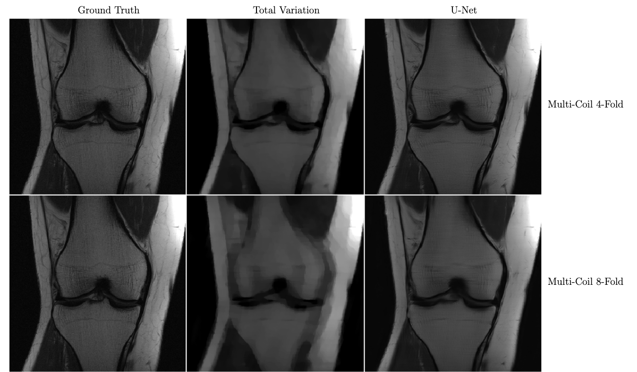
Knee MRI reconstructions comparison between compressed sensing with total variation regularization and the fastMRI U-Net baseline. The data is acquired using multiple coils at 4x and 8x subsampling. Reproduced from Zbontar et al. 2018.
VarNet
Instead of just feeding a physics-informed guess to a U-Net, VarNet uses the physics of MRI at multiple steps in its network (Sriram et al. 2020 & Hammernik et al. 2018). Recently, an interchangeability study of VarNet was done. It found that 1/4-th of the data with VarNet was diagnostically interchangeable with the ground truth reconstructions. In other words, radiologists made the same diagnoses with both methods! [Tell me a funny story about this study]
Below is a sample reconstruction from their study, compared with the ground truth. I can’t tell the difference.
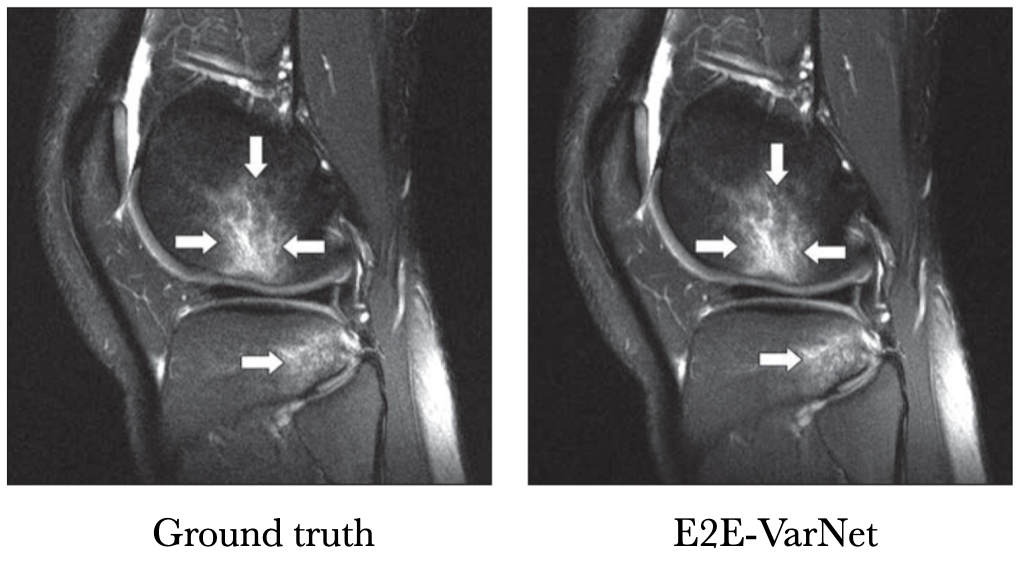
Knee MRI comparison between VarNet and the ground truth at 4x acceleration. Figure reproduced from Recht et al. 2020.
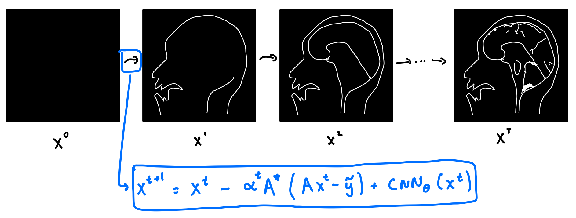
So how does VarNet work? It starts with a blank image, and consists of a series of refinement steps, progressively turning the blank image into a better and better version.
Let’s take a look at where the refinement step comes from. Recall that in classical compressed sensing, we solve the optimization problem above. Writing the forward operator $\mathbf{A}=\mathcal{M} \odot \mathcal{F}$, the optimization problem for compressed sensing becomes:
$$ \argmin_{\mathbf{x}} || \mathbf{A}\mathbf{x} - \mathbf{\tilde{y}} ||_2^2 + R(\mathbf{x})$$
This is not the optimization problem for VarNet, but we will use a cool trick called unrolled optimization:
If we solve the compressed sensing objective function via gradient descent, we get the following update equation for the $t$-th iteration of the image, ${\mathbf{x}}^t$.
$${\mathbf{x}}^{t+1} = {\mathbf{x}}^t - \alpha^t (\mathbf{A}^*(\mathbf{A}{\mathbf{x}}^t - \mathbf{\tilde{y}}) + \nabla R({\mathbf{x}}^t))$$
where $\mathbf{A}^*$ is the adjoint of $\mathbf{A}$. Note that gradient descent in the above equation is done on the image $\mathbf{x}$, as opposed to ${\boldsymbol{\theta}}$ . Now here’s the trick! Instead of hard coding the regularizer $R(\mathbf{x}^t)$, we can replace it with a neural network. We do this by replacing $\nabla R(\mathbf{x}^t)$ with a CNN. We get a new update equation:
$${\mathbf{x}}^{t+1} = {\mathbf{x}}^t - \alpha^t \mathbf{A}^*(\mathbf{A}{\mathbf{x}}^t - \mathbf{\tilde{y}}) + \text{CNN}_{\boldsymbol{\theta}} ({\mathbf{x}}^t)$$
The VarNet architecture consists of multiple layers. Each layer takes the output of the previous layer, ${\mathbf{x}}^t$, as its input, and outputs ${\mathbf{x}}^{t+1}$ according to the above equation. In practice, VarNet has about 8 layers, and the CNN is a U-Net. The parameters of the U-Net are updated via gradient descent on $\boldsymbol{\theta}$, and the loss function $\mathcal{L}({\boldsymbol{\theta}})$ is taken to be the structural similarity index measure (SSIM). [What is SSIM?]
Technically, the approach above isn’t quite the latest version of VarNet: there were a few changes that improve things a tiny bit. [What things?]
Deep Generative Priors
All methods above required access to a dataset that had both MRI images and the raw sensor data. However, to my understanding, the raw sensor data is not typically saved on clinical MRIs. Constructing a dataset with only the MRI images and without the raw sensor data might be easier. Fortunately, there are machine learning methods that only require MRI images as training data (i.e., unsupervised models).
One approach is to train what is called a generative model. Generative models are very popular in the computer vision community for generating realistic human faces or scenes (that it has never seen before!). Similarly, we can train a generative model to generate new MRI-like images.
A generative MRI model is a function $G_{\boldsymbol{\theta}}$ that tries to turn any random vector $\mathbf{z} \in \mathbb{R}^m$ into a realistic image $\mathbf{x} \in \mathbb{R}^n$. Typicaly, $m \ll n$, i.e., the input space is often much smaller than the output space.
Image reconstruction with generative models is done by solving the optimization problem: \begin{equation} \argmin_{\mathbf{z}} ||\mathbf{A} G_{\boldsymbol{\theta}}(\mathbf{z}) - \mathbf{\tilde{y}}||_2^2 \end{equation}
Instead of optimizing over all images $x \in \mathbb{R}^n$, we optimize only over the images produced by the generator, $G_{\boldsymbol{\theta}}(\mathbb{R}^m)$. Since $m \ll n$, the range of the generator $G_{\boldsymbol{\theta}}(\mathbb{R}^m)$ is much smaller than $\mathbb{R}^n$. [What if m=n?]
An important question is how well these models generalize outside of their training set. This is especially important for diagnosing rare conditions that might not appear in the training set. Jalal et al. 2021 recently showed that you can get pretty extraordinary generalization using a type of generative model called a score-based generative model. As seen in the results below, they train their model on brain data and test it on a completely different anatomy – in this case the abdomen! Their model performs much better in this case than other approaches.
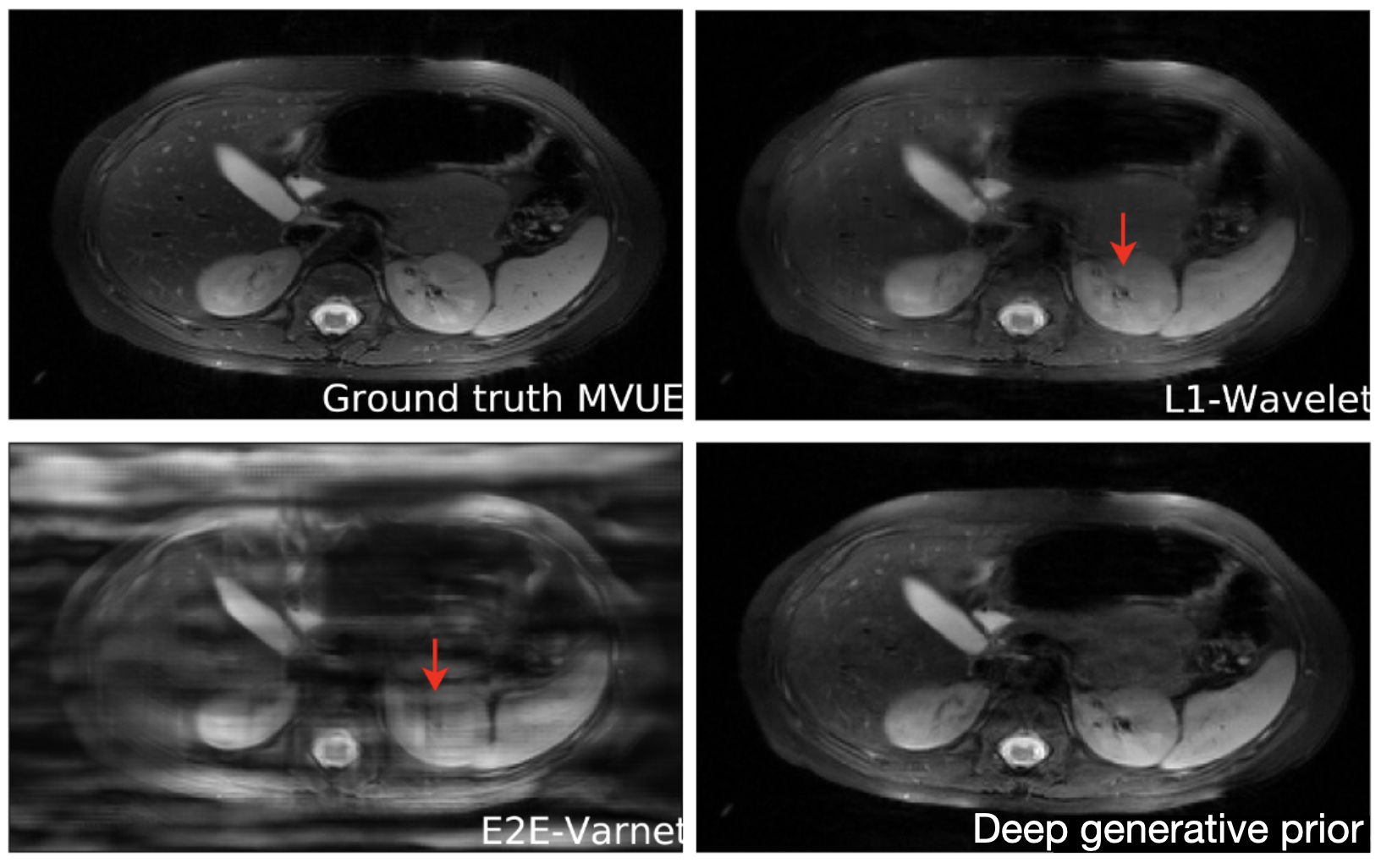
Reconstructions of 2D abdominal scans at 4x acceleration for methods trained on brain MRI data. The red arrows points to artifacts in the images. The deep generative prior method from Jalal 2021 does not have the artifacts from the other methods. Results from Jalal 2021.
Why generative models generalize so well, I don’t fully understand yet, but the authors do give some theoretical justification. A limitation to image reconstruction using deep generative priors is that the reconstruction time is typically longer than methods like VarNet (it can be more than 15 minutes on a modern GPU). This is because the optimization process needs to be run at test time.
Untrained Neural Networks
Imagine we get drunk again and forget to feed our machine learning model any data. We should get nonsense right…? Well, recently, it’s been shown that even with no data at all, the models in machine learning can be competitive with fully trained machine learning methods for MRI image reconstruction.
How do you explain this? First, let’s see how these models work. These no-data methods start with the deep generative priors approach in the previous section. But instead of using data to train the generator $G_{\boldsymbol{\theta}}(\mathbf{z})$, we set the parameters ${\boldsymbol{\theta}}$ randomly. The structure of these ML models – the fact that they’re made of convolutions, for example – make it such that without any data, realistic images are more likely to be generated than random noise.
This is remarkable! And confusing! We started off by saying that machine learning removes the need to manually engineer regularizers for compressed sensing. But instead, we are manually engineering the architectures of machine learning models! How much are these machine learning models really learning?
It turns out such untrained models have been applied to other inverse problems like region inpainting, denoising, and super resolution, and they have achieved remarkable results. Below are some results of an untrained model, ConvDecoder, on 4x subsampled data in MRI. We see that even though ConvDecoder is untrained, it produces better reconstructions than U-Net and TV-regularized compressed sensing.
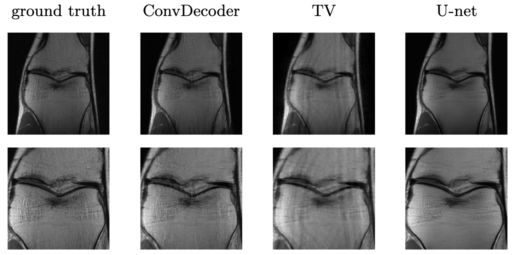
Comparison of the untrained ConvDecoder with the U-Net MRI, and total-variation regularized compressed sensing. Reconstructions of knee-MRI at 4x acceleration. The second row is a zoomed in version of the first row. Figure reproduced from Darestani et al. 2020.
Concluding Thoughts
Machine learning methods have made significant progress in reducing the scan time of MRI. Not only have ML methods for compressed sensing produced strong results on quantitative metrics like SSIM, but they have started to be validated by clinicians. Validation by clinicians is essential in image reconstruction because a fine detail can be essential in a diagnosis but might not make its way into a metric like the mean-squared-error.
A limitation to deep learning for healthcare is that we still don’t have a good understanding of why deep learning works. This makes it hard to predict when and how deep learning methods will fail (there are no theoretical guarantees that deep learning will work). One tool to help in this regard is uncertainty quantification: instead of only outputting a reconstructed image, you’d also output how much confidence you have in this image. Stochastic methods like deep generative priors can estimate the uncertainty in their reconstruction by creating many reconstructions with different random seeds and computing the standard deviation. For non-generative methods, works like Edupuganti 2019 make use of Stein’s unbiased risk estimate (SURE) to estimate uncertainty.
In addition to MRI, machine learning methods have also been used for other forms of image reconstruction. A great review can be found here.
A big thank you to Milan Cvitkovic, Stephen Fay, Jonathan Kalinowski, Hannah Le, and Marley Xiong for reviewing drafts of this.
This comes from two cool tricks in MRI, known as frequency encoding and phase encoding – maybe I will write a blog post on this. ↩︎
To be precise, MRI scan time scales linearly in 2 of the 3 spatial dimensions. We actually get one dimension of frequencies for free. This is from a neat trick known as frequency encoding which allows us to parallelize the acquisition process. ↩︎
Typically in machine learning, we use $\mathbf{x}$ to represent the input, and $\mathbf{y}$ as the output. But since image reconstruction is an “inverse problem,” we use the opposite notation. ↩︎